Skeleton analysis of a drosophila trachea

Skeleton analysis of a drosophila trachea#

In this notebook, we will study the elongated branching structure of a drosophila trachea in a 3D confocal image. We will introduce vesselness filters, skeletonization and show how the connected filaments structure can be represented as a graph of nodes and vertices using the Skan package in Python.

Acknowledgements

We kindly acknowledge Lemaitre lab in EPFL for providing the data for this notebook!

Setup#

Check that you have all the necessary packages installed, including napari and Skan. If not, you can use the ! symbol to install them directly from the Jupyter notebook (otherwise, you can use your terminal).

import napari
from skan import Skeleton, summarize

Get the data#

The image we’ll use in this tutorial is available for download on Zenodo (drosophila_trachea.tif).

In the cell below, we use a Python package called pooch to automatically download the image from Zenodo into the data folder of this repository.

import pooch
from pathlib import Path

data_path = Path('.').resolve().parent / 'data'
fname = 'drosophila_trachea.tif'

pooch.retrieve(
    url="https://zenodo.org/record/8099852/files/drosophila_trachea.tif",
    known_hash="md5:d595ac271779936e255afd0508cca43f",
    path=data_path,
    fname=fname,
    progressbar=True,
)

print(f'Downloaded image {fname} into: {data_path}')

Read the image#

We use the imread function from Scikit-image to read our TIF image.

from skimage.io import imread

image = imread(data_path / 'drosophila_trachea.tif')

print(f'Loaded image in an array of shape: {image.shape} and data type {image.dtype}')
print(f'Intensity range: [{image.min()} - {image.max()}]')

If you run into troubles, don’t hesitate to ask for help 🤚🏽.

Load the image into Napari#

Let’s open a viewer and load our image to have a look at it.

viewer = napari.Viewer(ndisplay=3)
viewer.add_image(image, name="Original image")

Intensity normalization#

Let’s rescale our image to the range 0-1. By doing so, it is also converted to an array of data type float.

from skimage.exposure import rescale_intensity

image_normed = rescale_intensity(image, out_range=(0, 1))

print(f'Intensity range: [{image_normed.min()} - {image_normed.max()}]')
print(f'Array type: {image_normed.dtype}')

Vesselness filtering#

Vesselness filters are designed to highlight elongated structures in an image. Here, we apply the meijering filter from Scikit-image to our normalized image.

from skimage.filters import meijering

image_mei = meijering(image_normed, sigmas=range(1, 3, 1), black_ridges=False)

# Have a look at what the filtered image looks like in Napari:
viewer.add_image(image_mei, name="Vesselness filter", contrast_limits=(0, 1));

Thresholding#

Next, we apply Otsu’s method to binarize the image.

from skimage.filters import threshold_otsu
import numpy as np

labels_binary = (image_mei >= threshold_otsu(image_mei)).astype(np.uint8)

# Have a look at the result
viewer.add_labels(labels_binary, name="Otsu threshold");

Skeletonization#

Finally, we use Scikit-image to skeletonize the image to extract a binary trace at the center of the filaments.

from skimage.morphology import skeletonize_3d

img_skeleton = skeletonize_3d(labels_binary)

viewer.add_image(
    img_skeleton, 
    name="Skeleton", 
    contrast_limits=(0, 1), 
    colormap='green', 
    blending='additive'
)

Analysis of the skeleton#

Using skan.Skeleton, we extract a graph representation of the skeleton in the form of a Pandas DataFrame.

table = summarize(Skeleton(skeleton_image=img_skeleton))

# Let's remove isolated branches (indexed as branch-type zero) from the table.
table.drop(table[table['branch-type'] == 0].index, axis=0, inplace=True)

table.head()

Visualization in Napari#

There is a little bit of extra work involved to prepare a vectors array of shape (N, 2, 3) suitable for Napari. Each row encodes the origin and end points of a 3D vector.

import pandas as pd

# Prepare the vectors for Napari
points_src = table[['image-coord-src-0', 'image-coord-src-1', 'image-coord-src-2']].values
points_dst = table[['image-coord-dst-0', 'image-coord-dst-1', 'image-coord-dst-2']].values

directions = points_dst - points_src

vectors = np.concatenate((points_src[np.newaxis], directions[np.newaxis]), axis=0)
vectors = np.swapaxes(vectors, 0, 1)

vectors.shape

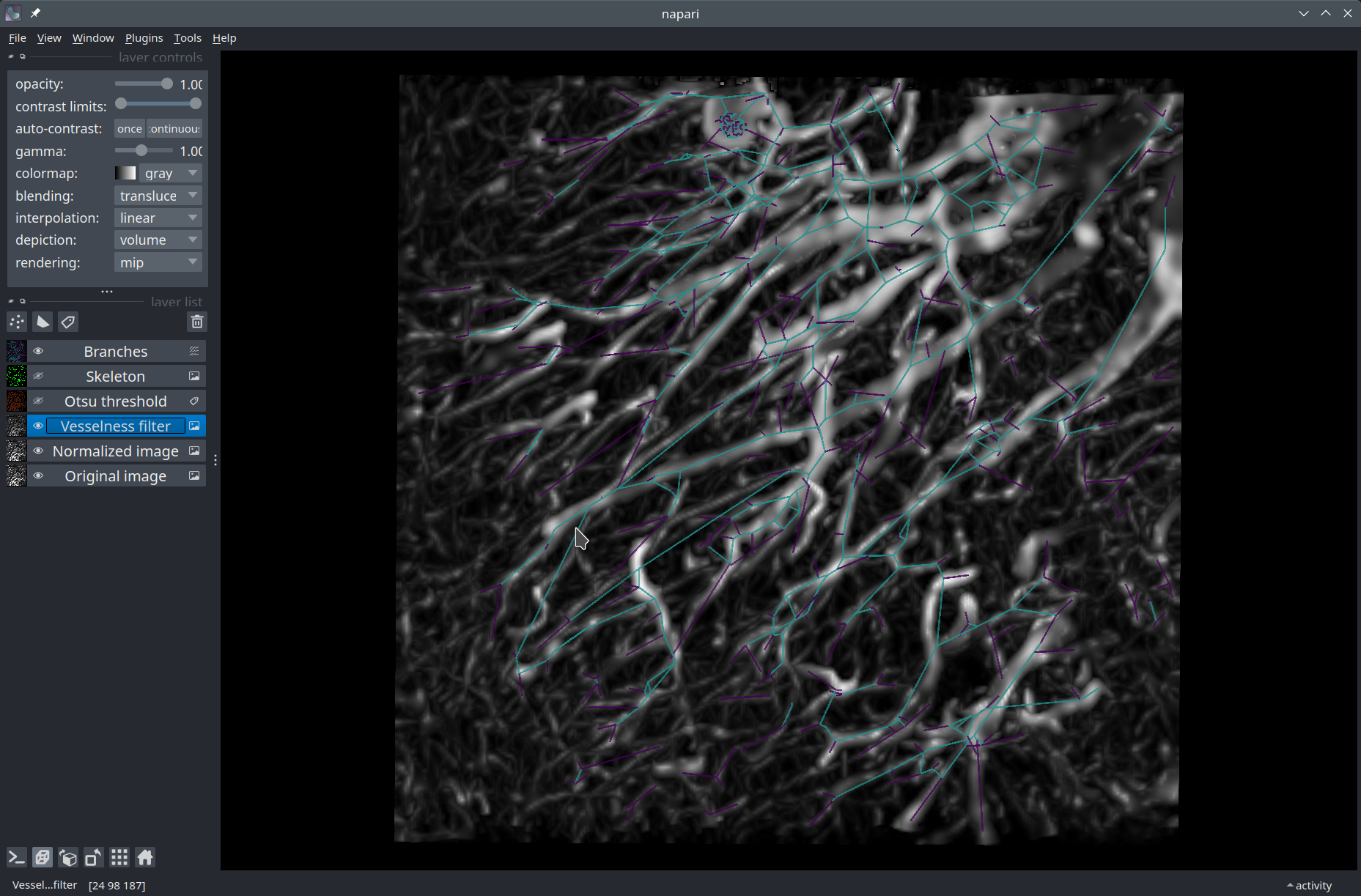
We can finally display our vectors in the viewer!

# Add a `Vectors` layer
viewer.add_vectors(vectors, name="Branches", edge_width=0.6, 
    features=pd.DataFrame({'branch-type': table['branch-type'].values.astype(float)}),
    edge_color='branch-type',
    vector_style='line',
)

Conclusion#

In this notebook, we have prototyped a way of extracting the skeleton of an elongated, fibrous structure in a scientific image. We used Napari’s Image, Labels, and Vectors layers to visualize the data resulting from processing the image.