Lungs convex hull detection

Lungs convex hull detection#

In this notebook, we will implement a simple image analysis pipeline to detect the area surrounding the lungs in the 3D CT scan of a mouse specimen.

Acknowledgements

We kindly acknowledge Prof. De Palma’s lab in EPFL for providing the data for this notebook!

Setup#

As usual, check that you have all the necessary packages installed.

import napari

Get the data#

The image we’ll use in this tutorial is available for download on Zenodo (lungs_ct.tif).

In the cell below, we use a Python package called pooch to automatically download the image from Zenodo into the data folder of this repository.

import pooch
from pathlib import Path

data_path = Path('.').resolve().parent / 'data'
fname = 'lungs_ct.tif'

pooch.retrieve(
    url="https://zenodo.org/record/8099852/files/lungs_ct.tif",
    known_hash="md5:80b294dc0a09fae7f861d0fa2bc7ab3c",
    path=data_path,
    fname=fname,
    progressbar=True,
)

print(f'Downloaded image {fname} into: {data_path}')

Read the image#

We use the imread function from Scikit-image to read our TIF image.

from skimage.io import imread

image = imread(data_path / 'lungs_ct.tif')

print(f'Loaded image in an array of shape: {image.shape} and data type {image.dtype}')
print(f'Intensity range: [{image.min()} - {image.max()}]')

If you run into troubles, don’t hesitate to ask for help 🤚🏽.

Load the image into Napari#

viewer = napari.Viewer()
viewer.add_image(image, name="Original image")

Intensity normalization#

Let’s rescale our image to the range 0-1. By doing so, it is also converted to an array of data type float.

from skimage.exposure import rescale_intensity

image_normed = rescale_intensity(image, out_range=(0, 1))

print(f'Intensity range: [{image_normed.min()} - {image_normed.max()}]')
print(f'Array type: {image_normed.dtype}')

# You can open the normalized image in Napari to inspect it!
viewer.add_image(image_normed, name="Normalized", contrast_limits=(0, 0.4))

Denoising#

You may have noticed that the original image is quite noisy.

A median filter will replace each pixel with the median value of its neighbors. This is an effective way of removing noisy pixels, which often have unusually high or low intensity values.

For more info, read: Median filtering (Cris Luengo).

from skimage.filters import median

denoised = median(image_normed)

# Look at the result in the viewer
viewer.add_image(denoised, name="Denoised", contrast_limits=(0, 0.4))

Interactively select a threshold for binarization#

There are several ways to set up custom interactions in Napari, one of which is by using the magicgui package. Read this page to learn more.

Below, we show how to integrate a simple Slider element to interactively threshold our image.

from napari.types import ImageData, LabelsData
from magicgui import magicgui

# The magicgui decorator converts a Python function to a GUI element (a slider).
@magicgui(auto_call=True, threshold={"widget_type": "FloatSlider", "max": 1})
def binary_thresold(layer: ImageData, threshold: float=0.5) -> LabelsData:
    """Applies a binary threshold to the image."""
    return (layer < threshold).astype('int')

# "Dock" the slider in the Napari viewer
viewer.window.add_dock_widget(binary_thresold, name="Median filter")

You should be able to move the slider in order to select a convenient intensity threshold for the lungs. Make sure to apply the threshold to the denoised image by selecting it in the dropdown list above the slider.

We found that a value of 0.1 works well for this image.

threshold = 0.1

binary = denoised < threshold

viewer.add_labels(binary)

Select the biggest object in the binary mask#

We assume that the biggest connected structure of pixels in the mask is the lungs. Let’s isolate it:

import numpy as np
from skimage.morphology import label

# First, we label the binary mask based on the connected components method
labels = label(binary)

# Count the number of pixels represented in each label
unique_labels, counts = np.unique(labels, return_counts=1)

# Ignore the background (labelled as zero) and find the index of the maximum count
biggest_label_idx = np.argmax(counts[1:]) + 1

biggest_label = unique_labels[biggest_label_idx]
print(f'Biggest label in the array is: {biggest_label} with {counts[biggest_label_idx]} pixels in it.')

# Extract the corresponding object mask
lungs_mask = (labels == biggest_label).astype(int)

# Visualize
viewer.add_labels(lungs_mask)

Convex hull#

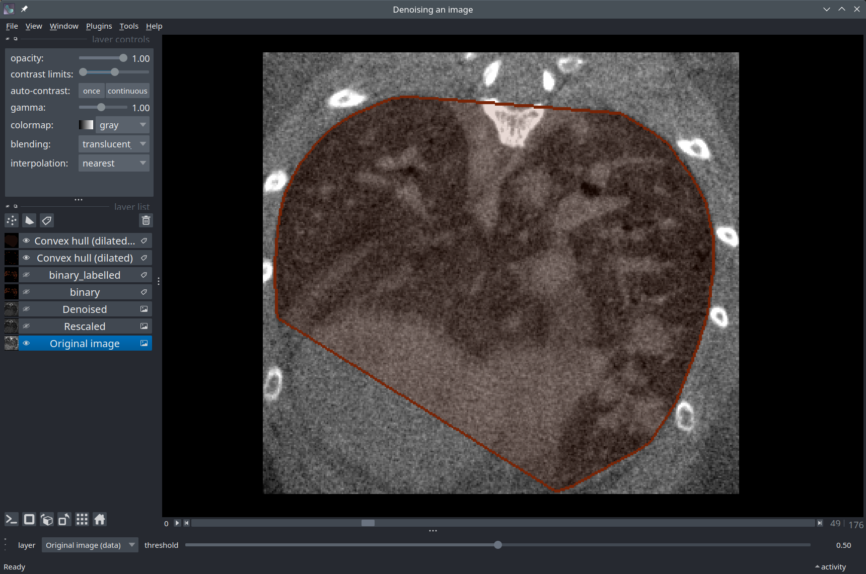
At this point, several strategies would be possible to further process the segmentation mask, depending on the needs. In the context of the project from which this example was taken, the goal is to generate a convex polygon that closely surrounds the lungs - a convex hull.

In the cell below, we use a function from Scikit-image to extract a convex hull separately in each 2D Z slice and we combine the results into a single 3D array using numpy.vectorize.

from skimage.morphology import convex_hull_image

hull = np.vectorize(convex_hull_image, signature='(n,m)->(n,m)')(lungs_mask)

hull_layer = viewer.add_labels(hull, name="Convex hull")

# The `contour` mode of a Labels layer only displays the edges of the mask:
hull_layer.contour = 2

Conclusion#

In this notebook, we have prototyped an image analysis pipeline to detect the area surrounding the lungs in a mouse CT scan. In doing so, we introduced the magicgui library, which can be used to implement customized, interactive user interface elements in Napari (such as a slider to dynamically threshold the image).